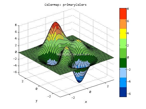
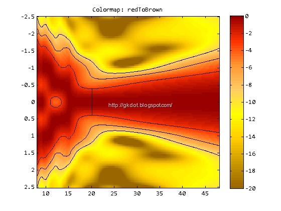
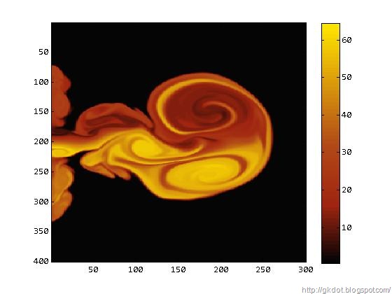
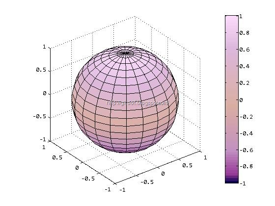
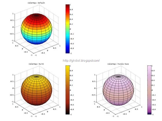
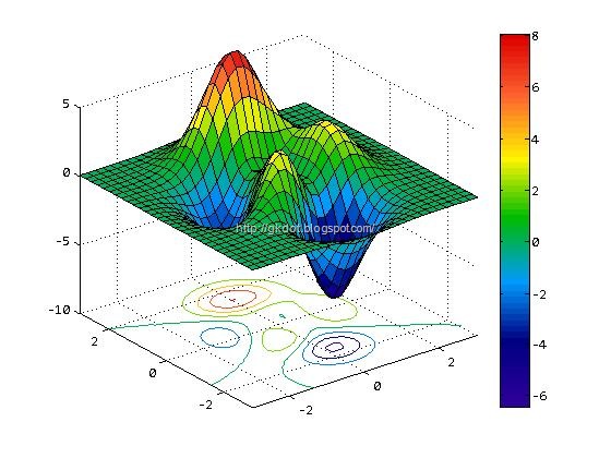
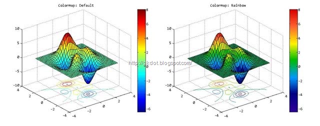
Colormap is a function (essentially a look-up table) that maps intensity to color. It is a very useful tool because with the right color map you can quickly convey information about particular aspects of an image.
Each colormap is comprised of 64 RGB triplets, each triplet taking values from 0 to 1 (instead of the typical 0 to 255; Why is that?). For examples see table below:
| Color | Red | Green | Blue |
| White | 1 | 1 | 1 |
| Red | 1 | 0 | 0 |
| Yellow | 1 | 1 | 0 |
| Blue | 0 | 0 | 1 |
MATLAB offers a number of color maps (I think 17 on R2008b) which are well thought out. My favorite maps are: default, bone, gray, hot. However, it is very easy to generate your own color maps in order to highlight (or mask) particular aspects of an image.
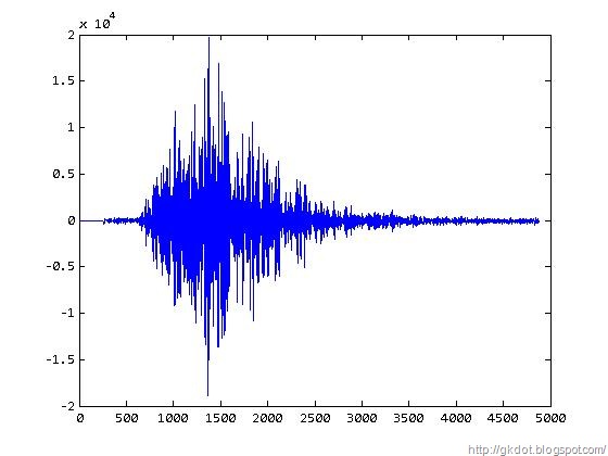
Say you have an RF signal (40 MHz sampling frequency) in vector x:
>> plot(x)

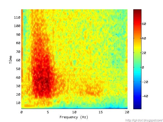
You can calculate the time - frequency spectrogram of the signal using the function spectrogram (which replaced the function specgram available in older releases; All these name changes are annoying.) Also use the function colorbar to display the current colormap.
>> spectrogram(x,256,240,256,40)
>> colorbar

The spectrogram is displayed with the default colormap which is very good for general purpose display of information. To change the colormap to another predefined one you can use the function colormap. For example:
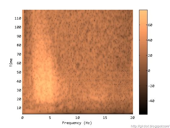
>> colormap(copper)

Too Flat. To go back to original colormap use:
>> colormap('default')
Note that to recall the default color map single quotes are need (for yet another unknown reason!)
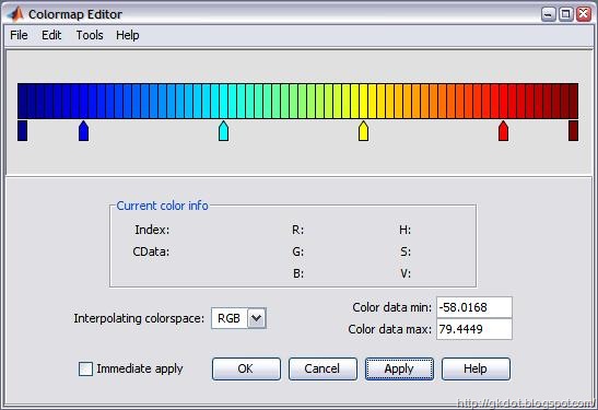
Frequently the predefined color maps are not sufficient to generate a useful graphic in a quantitative sense. MATLAB makes it very easy to generate custom maps by offering two possibilities: The one is to use the colormap editor GUI; The other is to do a bit of typing and use your brain at the same time!
To bring up the GUI type (obviously):
>> colormapeditor

You can do some cool stuff with the colormap GUI; The help menu has some good examples. The documentation is also available on-line here (but it is frequently slooowww; prefer the local help if it is installed).
However, GUIs are not exactly my thing. I prefer to keep my fingers on the keyboard. So here is what I would do:
Define number of colors in the colormap (as mentioned earlier that is a given).
>> n = 64;
Then define color nodes in realistic RGB color-per-row vectors. The first row specifies the one end of the colormap (in this example almost black) and the last row specifies the opposite end (in this example white). The rest of the rows define colors at specific points in the colormap. You do not need to define all 64 color explicitly (though that is not out of the question). Note that MATLAB does not know the standard RGB triplets so eventually they would have to be normalized (divided by 255).
>> nodes = [
10 0 0;
255 0 0;
255 255 0;
255 255 255
];
Define the index of each node in the colormap. The first row gets the index 1. The last row gets index 64. The index of the rest of the row vectors (or RGB triplets, or colors, or whatever) will define the rest of the color assignments in the colormap by interpolating between nodes.
>> index = [1 24 48 64];
In this case, index(24) is the 24th color of the colormap and is red ([255 0 0]) while index(48) is the 48th color of the colormap and is yellow ([255 255 0]).
Now we need to define the colors for all the other indices of the color map. There various ways to do that such 1st order polynomial fit per range, spline (not very good since it will introduce unwanted oscillations and thus values out-of-range that you need to take care off but creates some unique maps), etc. A decent way to go about it is to use the function linspace between nodes to create linearly spaced vectors. A first order fit it would be good but more typing!
>> RGBMap = zeros(n,3);
>> for id = 1:size(nodes,1)-1
for jd = 1:3
RGBMap(index(id):index(id+1),jd) = ...
round( ...
linspace(nodes(id,jd),nodes(id+1,jd),index(id+1)-index(id)+1) ) ./255;
end
end
>>
Note the division by 255 to change values from 0 to 1 to accommodate MATLAB weirdness.
Invoke map by typing:
>> colormap(RGBMap)
Where, RGBMap is the name of the color map parameter used here.
In this example the colormap is essentially identical to the MATLAB-defined colormap hot (can check using the colormap editor).
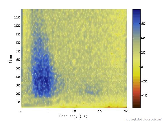
A colormap that I might have liked better would be:
>> nodes = [
45 25 0;
200 70 45;
215 215 20;
225 225 110;
170 180 120;
65 105 200;
25 25 125;
];
>> index = [1 11 22 32 43 55 64];
which would result to the following cleaner image:

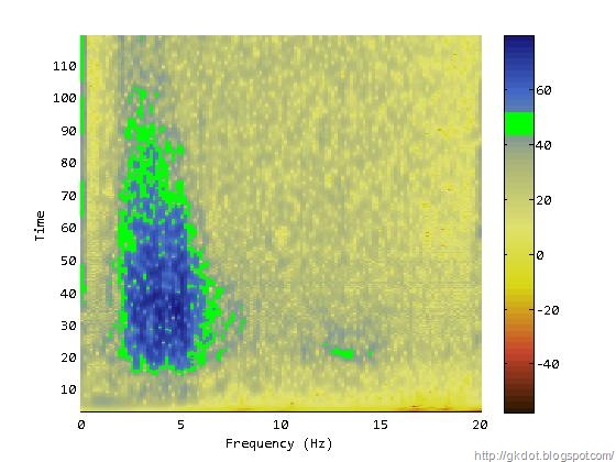
If I wanted to highlight a particular feature (a specific level) I could use:
>> nodes = [
45 25 0;
200 70 45;
215 215 20;
225 225 110;
170 180 120;
135 155 147;
0 255 0;
0 255 0;
91 124 180;
65 105 200;
25 25 125;
];
>> index = [1 11 22 32 43 47 48 51 52 55 64];

And of course I can relate the dB levels with the colormap and indices etc and produce really useful images.
